Introduction to Splines#

A general introduction to splines#

A spline is a very flexible and in particular smooth way of representing geometry. As such, splines have enjoyed great success in particular in design, be it engineering design or architecture. The following description is inspired by the books of Rogers as well as Piegl and Tiller (see section Further reading for the exact reference).

Splines come in many colors and facets, but there are a few properties that the most common ones (Bézier splines, B-splines, and NURBS) share:

Splines are parametric geometry descriptions. This means that each spline coordinate is expressed as a function of a local parameter. Assume that we are dealing with a spline curve, which is embedded in a two-dimensional space. Then the coordinates \((x,y)\) are computed as \((x(u),y(u))\), where \(u\) is the local parameter. An example could be \(x(u)=\cos(u),y(u)=\sin(u)\), which represents the unit circle. Usually, the local parameter is normalized, meaning that it takes on the value of \(0\) at one end of the curve and the value of \(1\) at the other end of the curve. Notice that parameterizations are not unique and one can represent the same geometry using different parameterizations.
The dimension of the geometric entity (i.e., 1D for a curve, 2D for a surface, 3D for a volume, etc.) determines the dimension of the parameter space. This means that a curve always has one local parameter, a curve two, etc.
In many cases, one is faced with so-called immersions, i.e., a spline of lower dimension is embedded into a higher-dimensional space, such as a curve into a 2D space. For this reason, the dimension of the parameter space (defined in \(\pmb{u}\)-coordinates) does not necessarily match the dimension of embedding space, which we will call the global space (defined in \(\mathbf{x}\)-coordinates).
The general equation for a spline curve \(\mathbf{S}\) is

\[\mathbf{S} = \sum_{i=1}^n N_i(u) \mathbf{P}\]

Here, \(N\) denotes the basis functions, \(\mathbf{P}\) the coordinates of the control points, and \(n\) the number of basis functions / control points. Geometrically, this means that one selects a certain number of points in the global space (i.e., the control points) and these points are “connected” using the basis functions. Notice that for splines, the basis functions can take on values within the interval \([0,1]\). However, they will usually never reach the value of one. As a consequence, the control points are not interpolated (meaning that the spline does not go through them), but they only guide the spline.

Higher-dimensional splines are derived from 1D-splines in a tensor-product fashion. This means that the control points are then arranged in structured grids and the basis functions are computed as a product of the univariate basis functions \(N_i(u)\) and \(M_j(\eta)\). Consider the example of a splines surface:

\[\mathbf{S}(u, \eta) = \sum_{i=1}^n \sum_{j=1}^m N_i(u) M_j(\eta) \mathbf{P}_{i,j}\]

Notice that the structure of \(N_i\) and \(M_j\) is exactly the same. They are simply defined in different coordinate directions.

In which situations are splines helpful?#

As previously mentioned, splines, or in particular non-uniform rational B-spline (NURBS), constitute the basis of computer aided design. However, this is not where the stories of splines ends. They are also very helpful in geometry representation for shape optimization, fitting of data points, but most of all, have become an important means also in numerical analysis. Here, we refer to the idea of isogeometric analysis (IGA), proposed by Hughes, Cottrell and Bazilevs in 2005.

An introduction to different spline types#

As described in the introduction, the principal structure of most spline types is the same. The only difference between the considered spline types are the definition of the basis functions \(N_i\). In the following, we will introduce the basis functions for four different spline types and discuss the specific properties they yield. We will restrict ourselves to the univariate basis functions and ask the reader to keep in mind that from there, one can derive the higher-dimensional basis functions as tensor products.

Bézier splines#

Named after Pierre Bézier (1910-1999), a French engineer at Renault and one of the founders of CAD/CAM systems, Bézier splines were one of the earliest spline representations. They use Bernstein polynomials as their basis function, which are defined as follows:

\[N_{i,p}(u)=\frac{(p)!}{(i-1)!(p+1-i)!}u^{i-1}(1-u)^{p+1-i} ,\]

with

\[ \begin{align}\begin{aligned}u &\in [0;1],\\0^{0} &\equiv 1,\\0! &= 1,\end{aligned}\end{align} \]

and the fixed relation between degree of the polynomial \(p\) and number of control points \(n\)

\[n=p+1 .\]

This means that the number of control points cannot be chosen freely, but is fixed the moment the degree has been chosen. Actually, this is a good moment to point to a terminology conflict that becomes very apparent, when geometers and analysts try to communicate: While a geometer uses the terms degree and order differently, assuming that order= degree+1, an analyst will tend to use those two terms interchangeably, meaning that order = degree.

After this basic definition, we will continue with a few examples.

Examples#

Example 1: Bézier curve with \(n=2\) control points and degree \(p=1\) In this case, there are two basis functions, both of degree \(1\). We denote the basis functions as \(N_{i,p}\), where \(i\) indicates the number of the basis function and \(p\) the degree of the basis function.

\[ \begin{align}\begin{aligned}N_{1,1}(u)&=\frac{1!}{0!1!}u^{0}(1-u)^{1}=1-u ,\\N_{2,1}(u)&=\frac{1!}{1!0!}u^{1}(1-u)^{0}=u .\end{aligned}\end{align} \]

The resulting spline curve can then be computed as follows:

\[\mathbf{S}(u)=(1-u)\mathbf{P}_{1}+u \mathbf{P}_{2} .\]

Example 2: Bézier curve with \(n=3\) control points and degree \(p=2\)

noindent In this case, there are three basis functions, all of degree \(2\).

\[ \begin{align}\begin{aligned}N_{1,2}(u)&=\frac{2!}{0!(2!)}u^{0}(1-u)^{2}=(1-u)^{2}\\N_{2,2}(u)&=\frac{2!}{1!(1!)}u^{1}(1-u)^{1}=2u (1-u)\\N_{3,2}(u)&=\frac{2!}{2!(0!)}u^{1}(1-u)^{0}=u^{2}\end{aligned}\end{align} \]

The resulting spline curve can then be computed as follows:

\[\mathbf{S}(u)=(1-u)^{2}\mathbf{P}_{1}+2u (1-u)\mathbf{P}_{2}+u^{2}\mathbf{P}_{3}\]

Properties of Bézier curves#

Bézier curves have the following properties:

The curve is contained in the convex hull of the control polygon (i.e. the largest convex polygon defined by the CPs).
The basis functions are real and (non-zero) throughout the entire definition space.
\(\mathbf{P}_{1}=\mathbf{S}(0)\) and \(\mathbf{P}_{n}=\mathbf{S}(1)\). This follows from:

\[ \begin{align}\begin{aligned}N_{1,p}(0)&=\underbrace{\frac{p!}{0!p!}}_{=1}\underbrace{0^{0}}_{=1}\underbrace{(1-0)^{p}}_{=1}=1\\N_{i,p}(0)&=\frac{p!}{(i-1)!p!}0^{i-1}(1-0)^{p+1-i}=0\qquad\text{if }i\neq 1\\C(0)&=1\cdot P_{1}\end{aligned}\end{align} \]

A similar argument can be made for \(\mathbf{P}_n\).

Bernstein polynomials form a partition of unity.

Drawbacks of Bézier curves#

In modern CAD systems, Bézier curves no longer play a role. This is due to two drawbacks:

Important types of curves cannot be represented using polynomials and thus also not with a Bézier spline, which has a polynomial basis. These include conic sections like circles, cylinders, cones, spheres, etc..
The control over the curve geometry is not sufficiently local (single segment curve). A high polynomial degree is required to satisfy a large number of constraints, i.e., complex shapes.

Rational Bézier splines#

One of the drawbacks of Bézier spline listed above is that it cannot be used to represent certain conic sections exactly. To this end, rational functions are needed. In this case, we will use rational functions defined via the ratio of two polynomials. The new basis function becomes:

\[R_{i,p}=\frac{N_{i,p}(u)\omega_{i}}{W(u)}=\frac{N_{i,p}(u)\omega_{i}}{\sum_{\hat{i}=1}^{n}N_{\hat{i},p}(u)\omega_{\hat{i}}} .\]

Here, \(N_{i,p}\) are the Bernstein polynomials discussed above. \(\omega_i\) is a so-called weight. \(\omega_i\) is greater than zero and provides a measure to scale the influence of a certain control point. If the weight tends to zero, the control point is technically excluded from the spline computation. If the weight becomes large, the spline moves very close to the respective control point. If all weights are equal, one retrieves a the Bézier spline (the weights cancel and the denominator than becomes zero due to the partition of unity property.

Properties of Rational Bézier splines#

The same properties of Bézier splines hold.

B-splines#

Just like the Bézier basis functions, B-spline basis functions are polynomials. The key difference is that they are non-zero in only a portion of the parameter space. In other words, the basis functions have local support and this is what, in contrast to Bézier splines, gives us local control over the spline. In order to indicate where the support of each basis function begins and ends, we define a series of break points. These break points are called knots. The collection of knots forms the knot vector \(u\):

\[u=[u_{1}=0,u_{2},\dots,u_{n}=1]\qquad \underbrace{0\le u\le 1}_{\text{ parameter space}} .\]

The entries of the knot vector form a non-decreasing sequence: \(u_{i}\le u_{i+1}\). It is however possible to repeat knot values. The interval \([u_{i},u_{i+1}]\) is called the \(i\)-th knot span. The length (meaning number of entries) of the knot vector, \(m\), is fixed as

\[ \begin{align}\begin{aligned}&m=n+p+1\\&n:\text{ number of basis functions/CPs}\\&p:\text{ degree} \nonumber\end{aligned}\end{align} \]

An example of a knot vector could be:

\[u=[0, 0, 0.5, 1, 1] .\]

It has a length of \(m=5\) and contains four knot spans. The first knot span is \([0,0]\) with a length of \(0\), the second knot span is \([0,0.5]\) with a length of \(0.5\), etc..

There are different types of knot vectors:

open \(\leftrightarrow\) periodic

In an open knot vector, the first and last value appears \(p+1\) times. A knot vector is called periodic, if it is not open. \(u=[0,0,0,0.5,1,1,1]\) is an open knot vector if \(p=2\).

uniform \(\leftrightarrow\) non-uniform In a uniform knot vector, the knots are equally spaced in the parameter space, e.g., \(u=[0,0.2,0.4,0.6,0.8,1]\). A knot vector is called non-uniform, if this condition is not fulfilled. An exception to this rule are repeated knot values in the beginning or end of the knot vector, e.g., \([0,0,0,0.5,1,1,1]\). This knot vector is then still called uniform, if all middle knots are equally spaced.

Once the knot vector has been specified, the basis functions \(N_{i,p}\) can be defined. Again, \(i\) indicates the number of the basis function and \(p\) the degree. \(N_{i,p}\) is defined by the Cox-de Boor recurrence formula. The starting point are constant basis functions (\(p=0\)) defined as follows:

\[\begin{split}N_{i,0}(u)= \begin{cases} 1, & \quad u_{i}\le u < u_{i+1} \qquad (i\text{th knot span}), \\\\ 0, & \quad \text{otherwise.} \end{cases}\end{split}\]

Subsequently, the degree of the basis function can be raised bit by bit using

\[N_{i,p}(u)=\frac{u-u_{i}}{u_{i+p}-u_{i}}N_{i,p-1}(u)+\frac{u_{i+p+1}-u}{u_{i+p+1}-u_{i+1}}N_{i+1,p-1}(u) ,\]

until the desired degree has been reached.

Properties of B-spline basis functions:#

constitute a partition of unity \(\sum_{i=1}^{n}N_{i,p}(u)=1\)
non-negative
continuously differentiable within knot spans, \(p-k\) times continuously differentiable across knots (\(k\): multiplicity of knot)
computation of a set of basis functions requires a knot vector \(u\) and a degree \(p\)
basis functions are non-zero in \([u_{i},u_{i+p+1})\), i.e., in \(p+1\) knot spans
in each knot span, \(p+1\) basis function will be nonzero
each basis function attains exactly one maximum in the interval \([u_{p+1},u_{n+1}]\), except for the case \(p=0\)
if the number of basis functions is \(p+1\), the B-spline basis reduces to the Bézier basis

Non-uniform rational B-splines (NURBS)#

In an argument similar to rational Bézier splines, NURBS are the rational counterpart of B-splines. In fact, a NURBS entity in \(\mathbb{R}^{d}\) is obtained by the projective transformation of a B-spline entity in \(\mathbb{R}^{d+1}\).

The NURBS basis functions \(R_{i,p}\) are computed using the B-spline basis functions \(N_{i,p}\):

\[R_{i,p}=\frac{N_{i,p}(u)\omega_{i}}{W(u)}=\frac{N_{i,p}(u)\omega_{i}}{\sum_{\hat{i}=1}^{n}N_{\hat{i},p}(u)\omega_{\hat{i}}} .\]

Again, \(\omega_i\) is a weight.

Properties of NURBS basis functions:#

The same properties of B-spline basis functions hold with the following additions:

computation of a set of basis functions additionally requires the weights \(\{\omega_i\}\)
if all weights are equal (\(\omega_i=a\) for all \(i\) and arbitrary \(a \neq 0\)), the NURBS basis reduces to the B-spline basis

Spline visualization#

Visualization#

One of the highlights of splinepy is that we can visualize splines. Most of the classes have their own show() function to visualize current state of each object. Visualizations utilize mesh types and data structures of gustaf. Then, actual rendering happens with vedo - a powerful scientific analysis and visualization library - check them out for details!

The following will give a brief introduction to spline visualization.

Creating a basic NURBS#

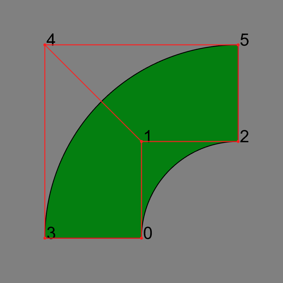
Here, we start by creating a NURBS object with array-like inputs.

import splinepy

# Initialize nurbs with any array-like input
nurbs = splinepy.NURBS(
    degrees=[2, 1],
    knot_vectors=[
        [0, 0, 0, 1, 1, 1],
        [0, 0, 1, 1],
    ],
    control_points=[
        [-1.0, 0.0],
        [-1.0, 1.0],
        [0.0, 1.0],
        [-2.0, 0.0],
        [-2.0, 2.0],
        [0.0, 2.0],
    ],
    weights=[
        [1.0],
        [2**-0.5],
        [1.0],
        [1.0],
        [2**-0.5],
        [1.0],
    ],
)

# vizusalize
nurbs.show()

Setting show_options#

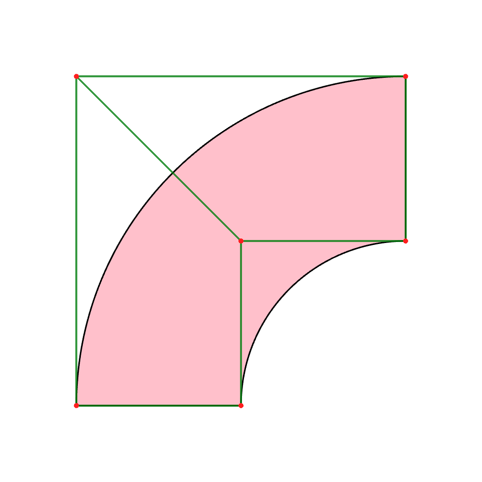
You can also customize visualization by setting *show_options*:

nurbs.show_options["c"] = "pink"
nurbs.show_options["control_point_ids"] = False

# You can use `update()` to set multiple options at once
# As visualization runs through mesh based engines, you can set sampling
# resolutions per dimension.
# In case of int, it will apply that for all dimension
nurbs.show_options.update(control_mesh_c="green", resolutions=[201, 3])

nurbs.show()

Plotting data on spline#

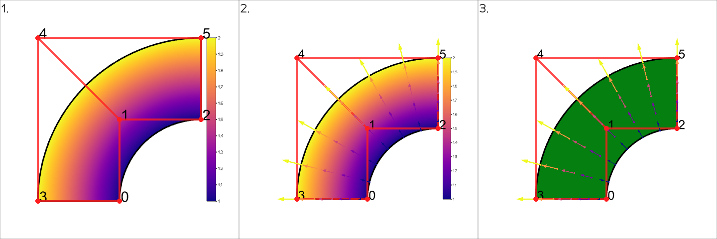
You can easily plot data on splines. Scalar data can be represented with a colormap and vector data can be represented with arrows. You can take a look at this example for detailed introduction.

# set data - we will plot self spline, which will plot coordinates
nurbs.spline_data["coords"] = nurbs

# then, set in show_options the name of the data
# "data" keyword will process any data as scalar - in case of vector data,
# it will take the norms
nurbs.show_options["data"] = "coords"
nurbs.show_options["scalarbar3d"] = True
nurbs.show()  # Nr. 1

# at the same time, you can plot vector data
# the keyword here is "arrow_data"
nurbs.show_options["arrow_data"] = "coords"

# by default, this will place an arrow at each sampling location which most of
# the time is too many. With "arrow_data_on", you can specify locations
nurbs.show_options["arrow_data_on"] = splinepy.uniform_query(
    nurbs.parametric_bounds, [7, 5]
)
nurbs.show()  # Nr. 2

# to turn off, just set None or pop()
nurbs.show_options.pop("data")
nurbs.show()  # Nr. 3

Examples#

Take a look at the examples folder for more!

Notebook plotting#

You can also plot your splines inside a notebook. For this you need to change the vedo backend to ‘k3d’. To do this you need to add the following lines to the top of the notebook.

import vedo

vedo.settings.default_backend = "k3d"

After this most functionality of the normal plotting should be available to you. Please write an issue if you find something that you can plot in a script but not in a notebook. There is one known issue regarding number of Line objects that we can plot (limited to 200 from vedo). We are working on a solution, but meanwhile, plotting curves is limited to resolutions of 201; for 2D/3D splines you can turn off knots in show_options. An example is provided in the folder examples/ipynb.

List of show_options#

SplineShowOption#

Color in {rgb, RGB, str of (hex, name), int}

allowed types: ( str, tuple, list, int)
default: None

alpha

Transparency in range [0, 1].

allowed types: ( float, int)
default: None

data

Name of vertex_data to show. Object must have vertex_data with the same name.

allowed types: ( str,)
default: None

vertex_ids

Show ids of vertices

allowed types: ( bool,)
default: None

element_ids

Show ids of elements

allowed types: ( bool,)
default: None

lighting

Lighting options {‘default’, ‘metallic’, ‘plastic’, ‘shiny’, ‘glossy’, ‘ambient’, ‘off’}

allowed types: ( str,)
default: None

cmap

Colormap for vertex_data plots.

allowed types: ( str,)
default: None

vmin

Minimum value for cmap

allowed types: ( float, int)
default: None

vmax

Maximum value for cmap

allowed types: ( float, int)
default: None

cmap_alpha

Colormap Transparency in range [0, 1].

allowed types: ( float, int)
default: None

cmap_n_colors

Set the number of available colors

allowed types: ( int,)
default: None

scalarbar

Scalarbar describing cmap. At least an empty dict or dict with following items are accepted: {title: str, pos: tuple, title_yoffset: int, font_size: int, nlabels: int, c: str, horizontal: bool, use_alpha: bool, label_format: str}. Setting bool will add a default scalarbar

allowed types: ( bool, dict)
default: None

scalarbar3d

3D scalarbar describing cmap. At least an empty dict or dict with following items are accepted: {title: str, pos: tuple, size: list, title_font: str, title_xoffset: float, title_yoffset: float, title_size: float, title_rotation: float, nlabels: int, label_font:str, label_size: float, label_offset: float, label_rotation: int, label_format: str, draw_box: bool, above_text: str, below_text: str, nan_text: str, categories: list}

allowed types: ( bool, dict)
default: None

arrow_data

Name of vertex_data to plot as arrow. Corresponding data should be at least 2D. If you want more control over arrows, consider creating edges using gus.create.edges.from_data().

allowed types: ( str,)
default: None

arrow_data_scale

Scaling factor for arrow data.

allowed types: ( float, int)
default: None

arrow_data_color

Color for arrow data. Can be either cmap name or color. For cmap, colors are based on the size of the arrows.

allowed types: ( str, tuple, list, int)
default: None

axes

Configure a specific axes with options. Expect dict(), but setting True will set a default axes. For full options, see https://vedo.embl.es/autodocs/content/vedo/addons.html#vedo.addons.Axes

allowed types: ( bool, dict)
default: None

knots

Show spline’s knots.

allowed types: ( bool,)
default: None

knot_c

Knot color.

allowed types: ( str, tuple, list, int)
default: None

knot_lw

Line width of knots. Number of pixels. Applicable to para_dim > 1.

allowed types: ( float, float)
default: None

knot_alpha

Transparency of knots in range [0, 1]. Applicable to para_dim > 1

allowed types: ( float, int)
default: None

control_points

Show spline’s control points.Options propagates to control mesh, unless it is specified.

allowed types: ( bool,)
default: None

control_point_r

Control point radius

allowed types: ( float, int)
default: None

control_point_c

Color of control_points in {rgb, RGB, str of (hex, name), int}

allowed types: ( str, tuple, list, int)
default: None

control_point_alpha

Transparency of control points in range [0, 1].

allowed types: ( float, int)
default: None

control_point_ids

Show ids of control_points.

allowed types: ( bool,)
default: None

control_mesh

Show spline’s control mesh.

allowed types: ( bool,)
default: None

control_mesh_c

Color of control_mesh in {rgb, RGB, str of (hex, name), int}

allowed types: ( str, tuple, list, int)
default: None

control_mesh_lw

Line width of control mesh. Number of pixels

allowed types: ( float, int)
default: None

resolutions

Sampling resolution for spline.

allowed types: ( int, list, tuple, numpy.ndarray)
default: None

Line width 1D spline.Applicable to para_dim > 1.

allowed types: ( float, int)
default: None

fitting_queries

Shows fitting queries if they are locally saved in splines.

allowed types: ( bool,)
default: None

arrow_data_on

Specify parametric coordinates to place arrow_data.

allowed types: ( list, tuple, numpy.ndarray)
default: None

MultipatchShowOption#

Color in {rgb, RGB, str of (hex, name), int}

allowed types: ( str, tuple, list, int)
default: None

alpha

Transparency in range [0, 1].

allowed types: ( float, int)
default: None

data

Name of vertex_data to show. Object must have vertex_data with the same name.

allowed types: ( str,)
default: None

vertex_ids

Show ids of vertices

allowed types: ( bool,)
default: None

element_ids

Show ids of elements

allowed types: ( bool,)
default: None

lighting

Lighting options {‘default’, ‘metallic’, ‘plastic’, ‘shiny’, ‘glossy’, ‘ambient’, ‘off’}

allowed types: ( str,)
default: None

cmap

Colormap for vertex_data plots.

allowed types: ( str,)
default: None

vmin

Minimum value for cmap

allowed types: ( float, int)
default: None

vmax

Maximum value for cmap

allowed types: ( float, int)
default: None

cmap_alpha

Colormap Transparency in range [0, 1].

allowed types: ( float, int)
default: None

cmap_n_colors

Set the number of available colors

allowed types: ( int,)
default: None

scalarbar

allowed types: ( bool, dict)
default: None

scalarbar3d

allowed types: ( bool, dict)
default: None

arrow_data

Name of vertex_data to plot as arrow. Corresponding data should be at least 2D. If you want more control over arrows, consider creating edges using gus.create.edges.from_data().

allowed types: ( str,)
default: None

arrow_data_scale

Scaling factor for arrow data.

allowed types: ( float, int)
default: None

arrow_data_color

Color for arrow data. Can be either cmap name or color. For cmap, colors are based on the size of the arrows.

allowed types: ( str, tuple, list, int)
default: None

axes

Configure a specific axes with options. Expect dict(), but setting True will set a default axes. For full options, see https://vedo.embl.es/autodocs/content/vedo/addons.html#vedo.addons.Axes

allowed types: ( bool, dict)
default: None

knots

Show spline’s knots.

allowed types: ( bool,)
default: None

knot_c

Knot color.

allowed types: ( str, tuple, list, int)
default: None

knot_lw

Line width of knots. Number of pixels. Applicable to para_dim > 1.

allowed types: ( float, float)
default: None

knot_alpha

Transparency of knots in range [0, 1]. Applicable to para_dim > 1

allowed types: ( float, int)
default: None

control_points

Show spline’s control points.Options propagates to control mesh, unless it is specified.

allowed types: ( bool,)
default: None

control_point_r

Control point radius

allowed types: ( float, int)
default: None

control_point_c

Color of control_points in {rgb, RGB, str of (hex, name), int}

allowed types: ( str, tuple, list, int)
default: None

control_point_alpha

Transparency of control points in range [0, 1].

allowed types: ( float, int)
default: None

control_point_ids

Show ids of control_points.

allowed types: ( bool,)
default: None

control_mesh

Show spline’s control mesh.

allowed types: ( bool,)
default: None

control_mesh_c

Color of control_mesh in {rgb, RGB, str of (hex, name), int}

allowed types: ( str, tuple, list, int)
default: None

control_mesh_lw

Line width of control mesh. Number of pixels

allowed types: ( float, int)
default: None

resolutions

Sampling resolution for spline.

allowed types: ( int, list, tuple, numpy.ndarray)
default: None

Line width 1D spline.Applicable to para_dim > 1.

allowed types: ( float, int)
default: None

Introduction to Splines#

A general introduction to splines#

In which situations are splines helpful?#

An introduction to different spline types#

Bézier splines#

Examples#

Properties of Bézier curves#

Drawbacks of Bézier curves#

Rational Bézier splines#

Properties of Rational Bézier splines#

B-splines#

Properties of B-spline basis functions:#

Non-uniform rational B-splines (NURBS)#

Properties of NURBS basis functions:#

Further reading#

Spline visualization#

Visualization#

Creating a basic NURBS#

Setting show_options#

Plotting data on spline#

Examples#

Notebook plotting#

List of show_options#

SplineShowOption#

MultipatchShowOption#